Benchmarks

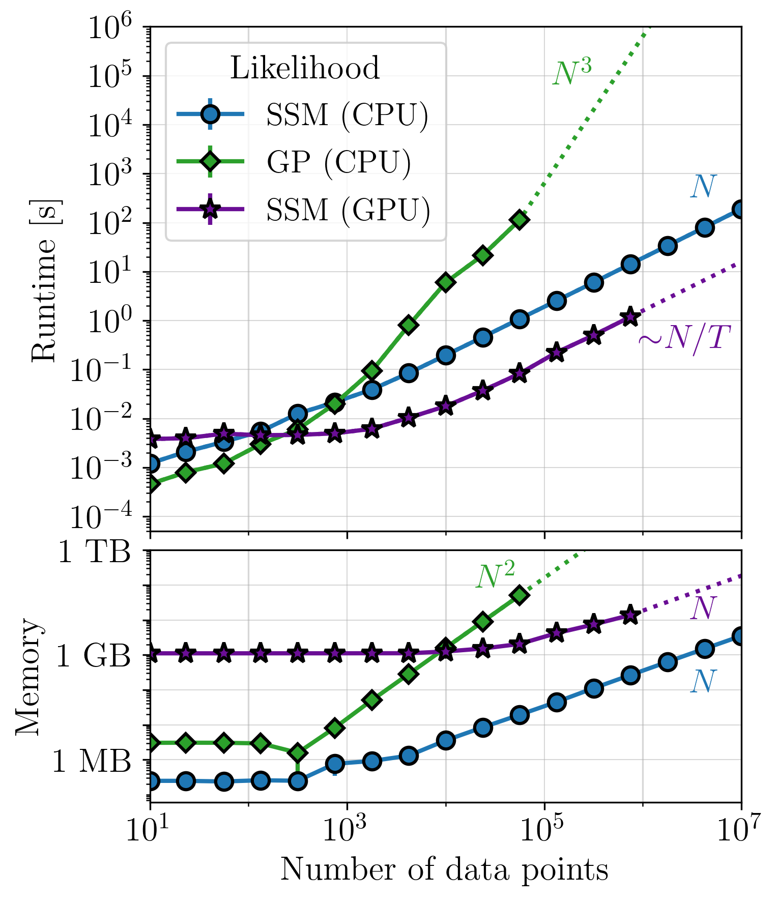
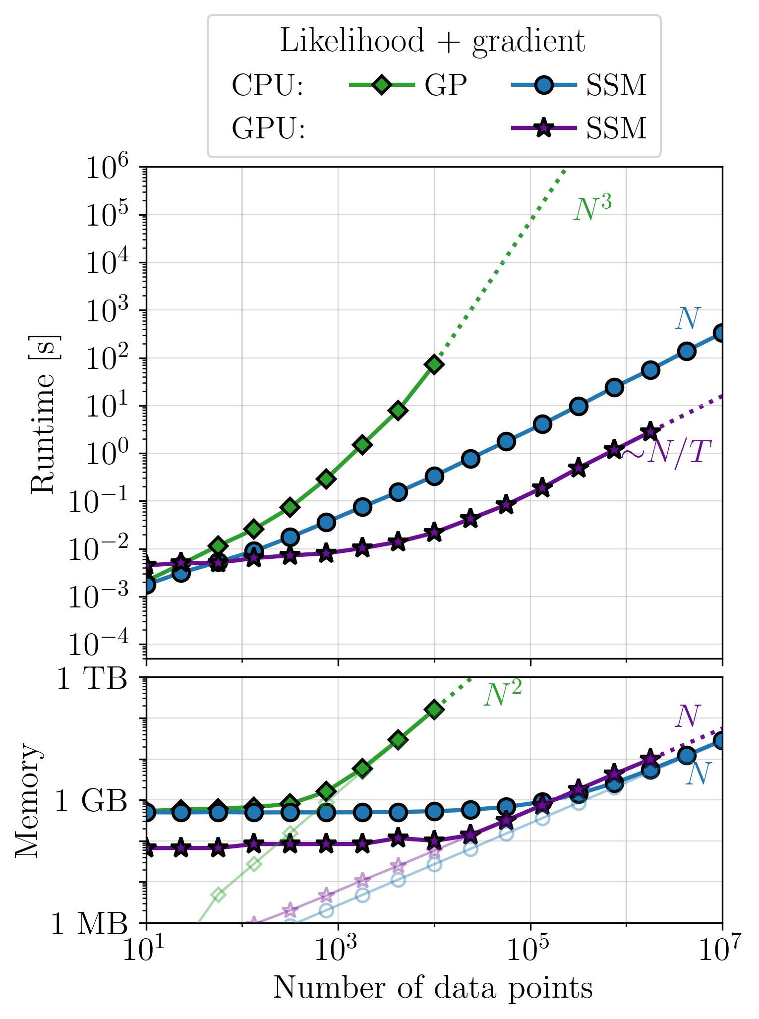
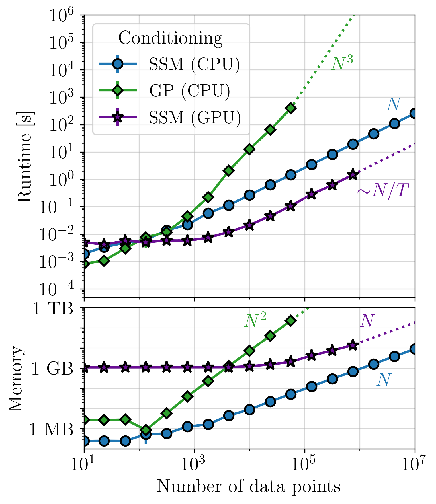
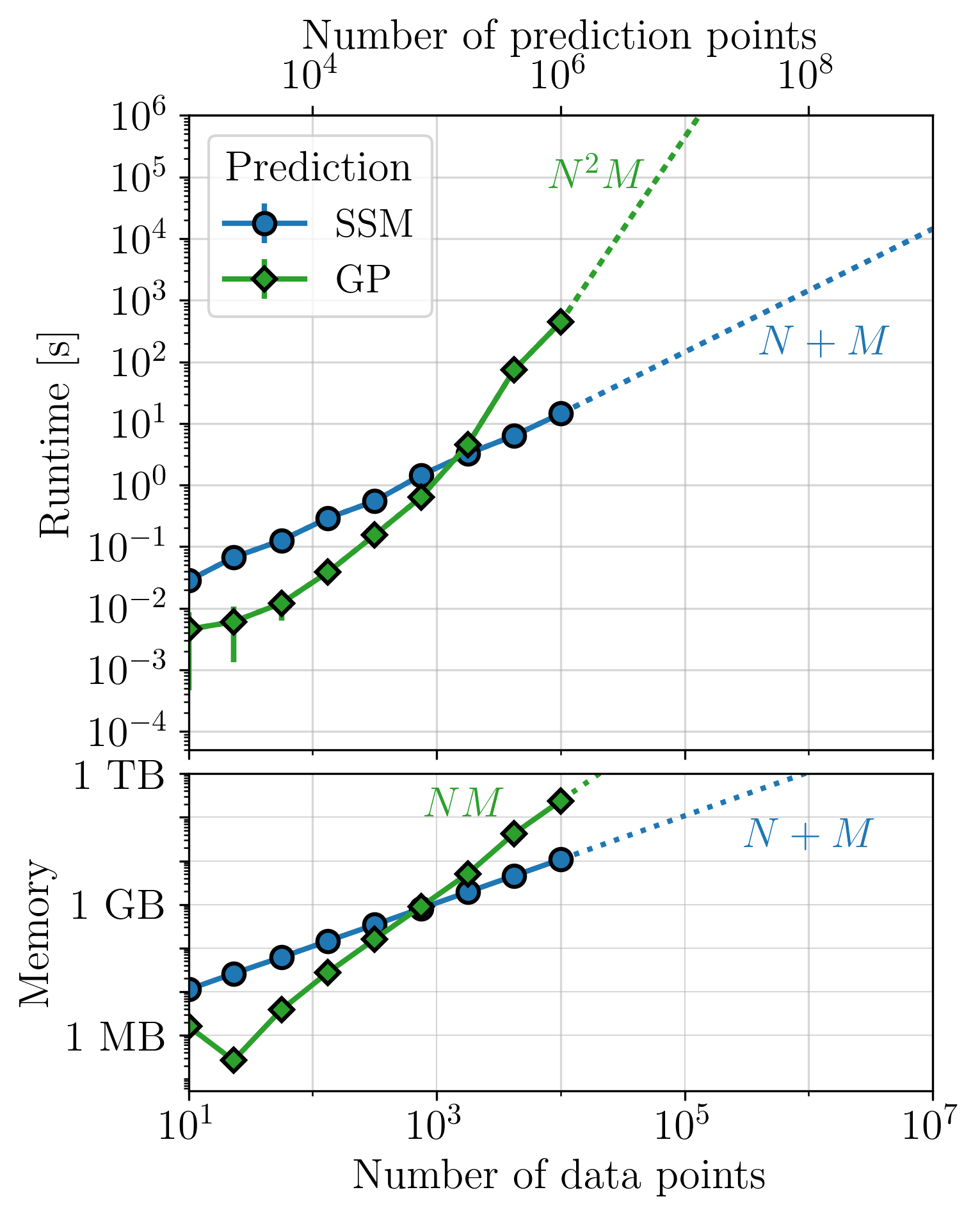
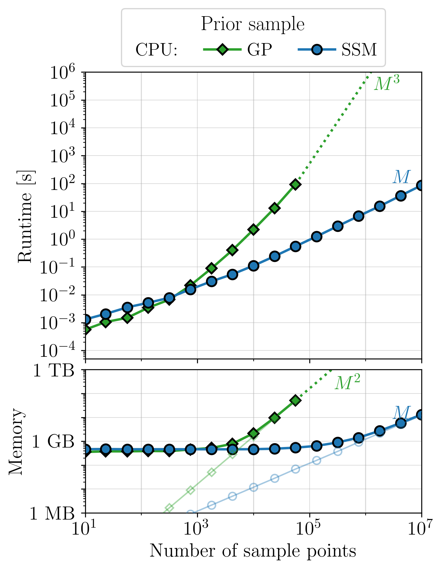
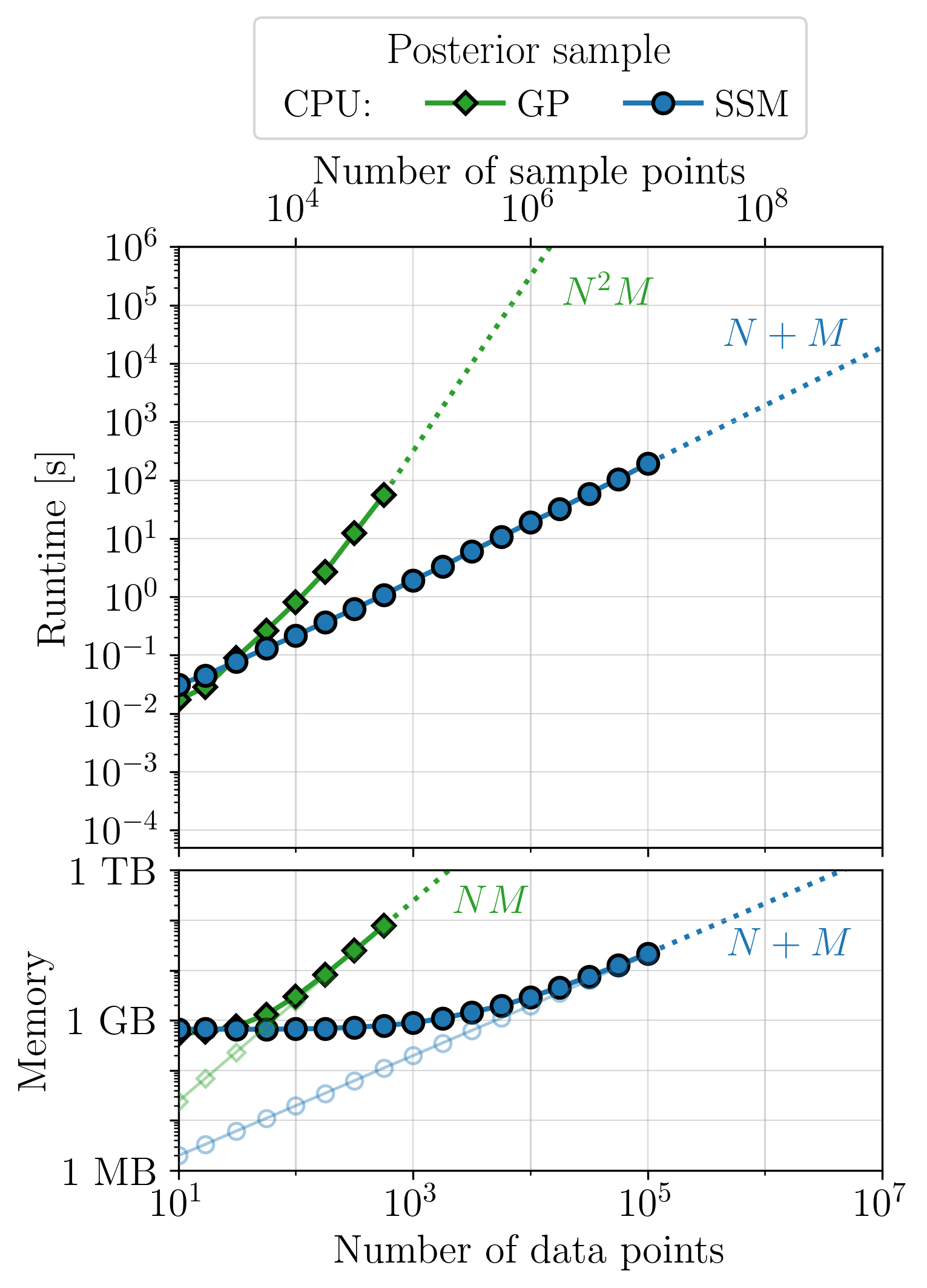
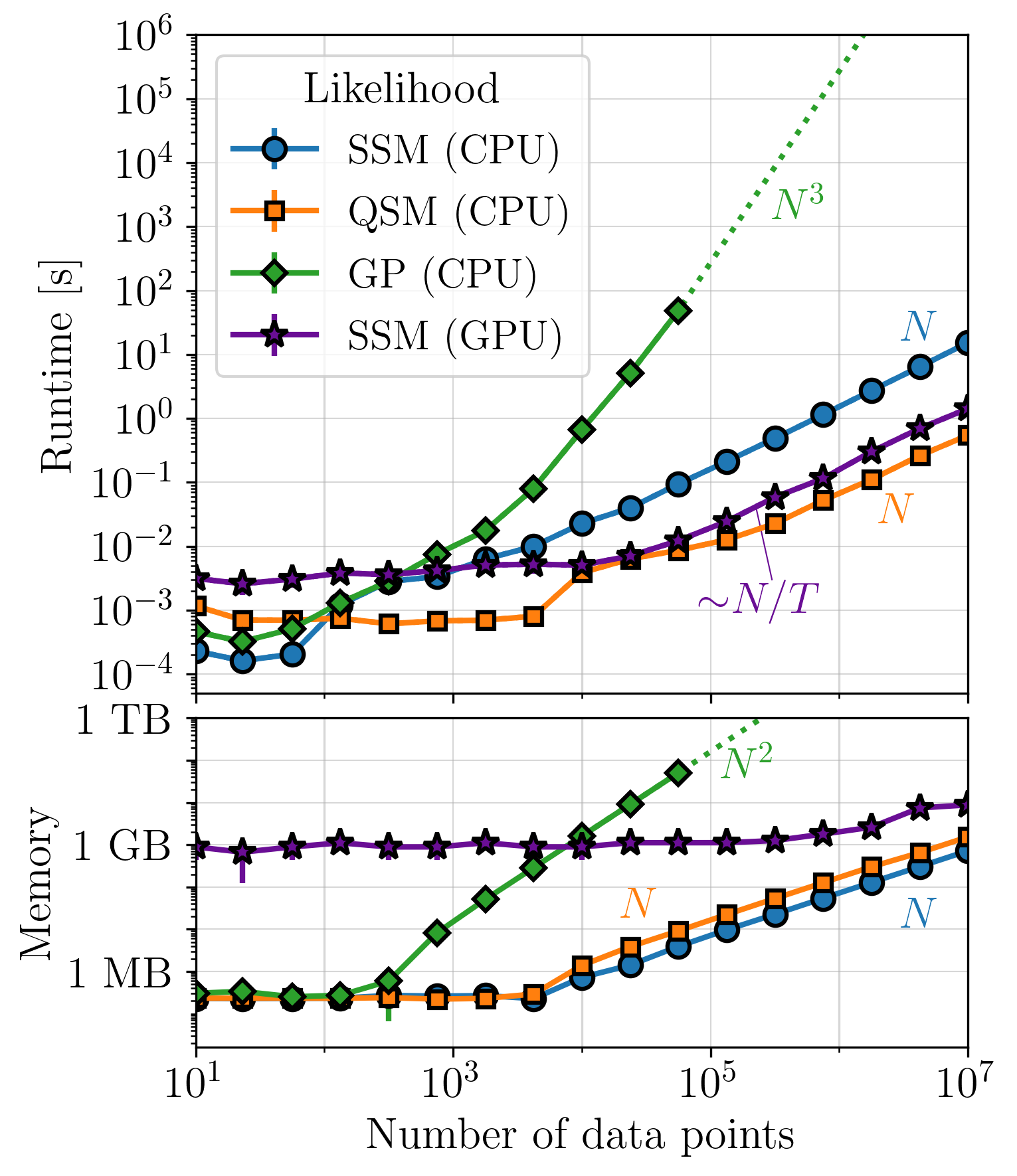
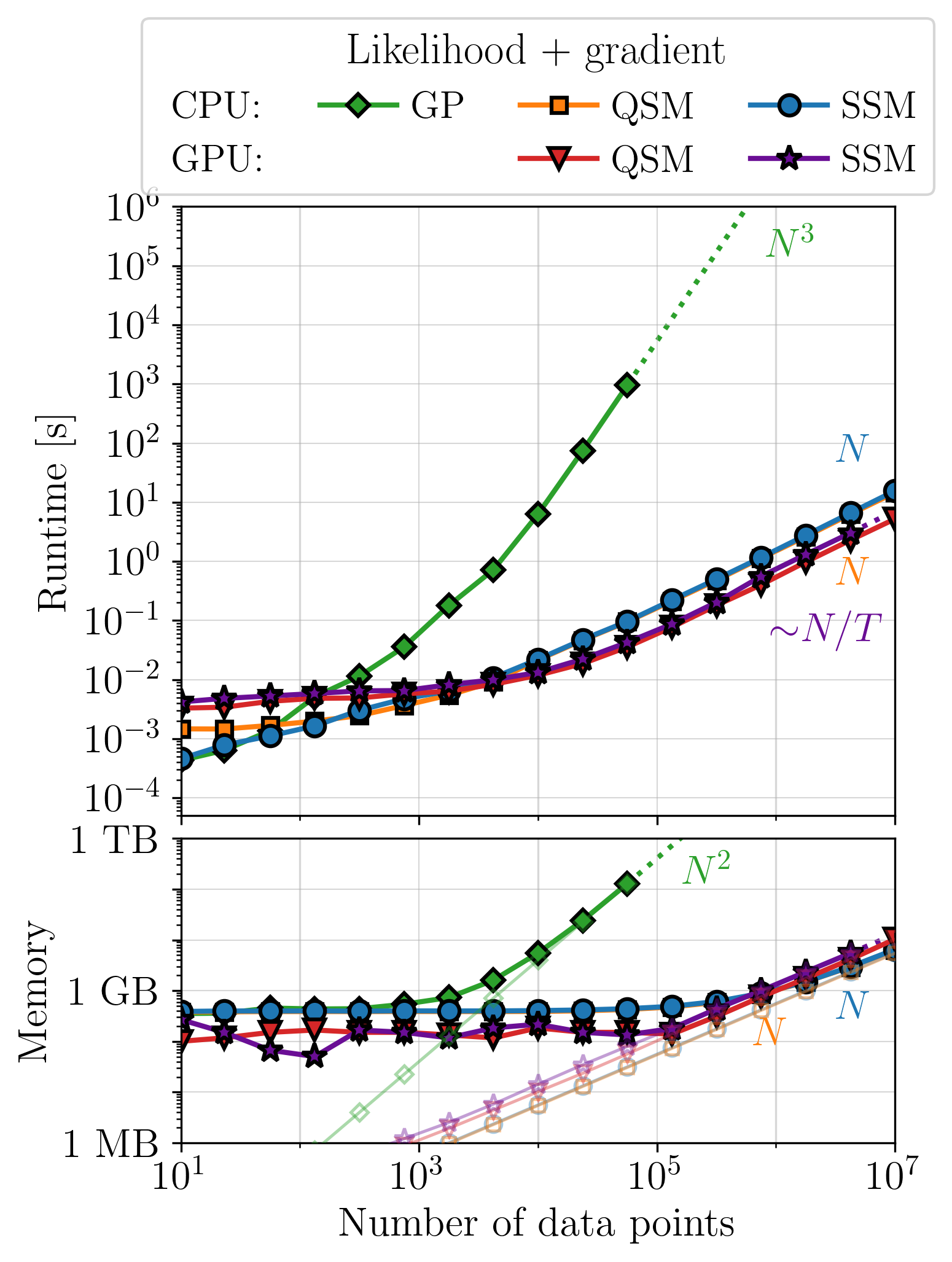
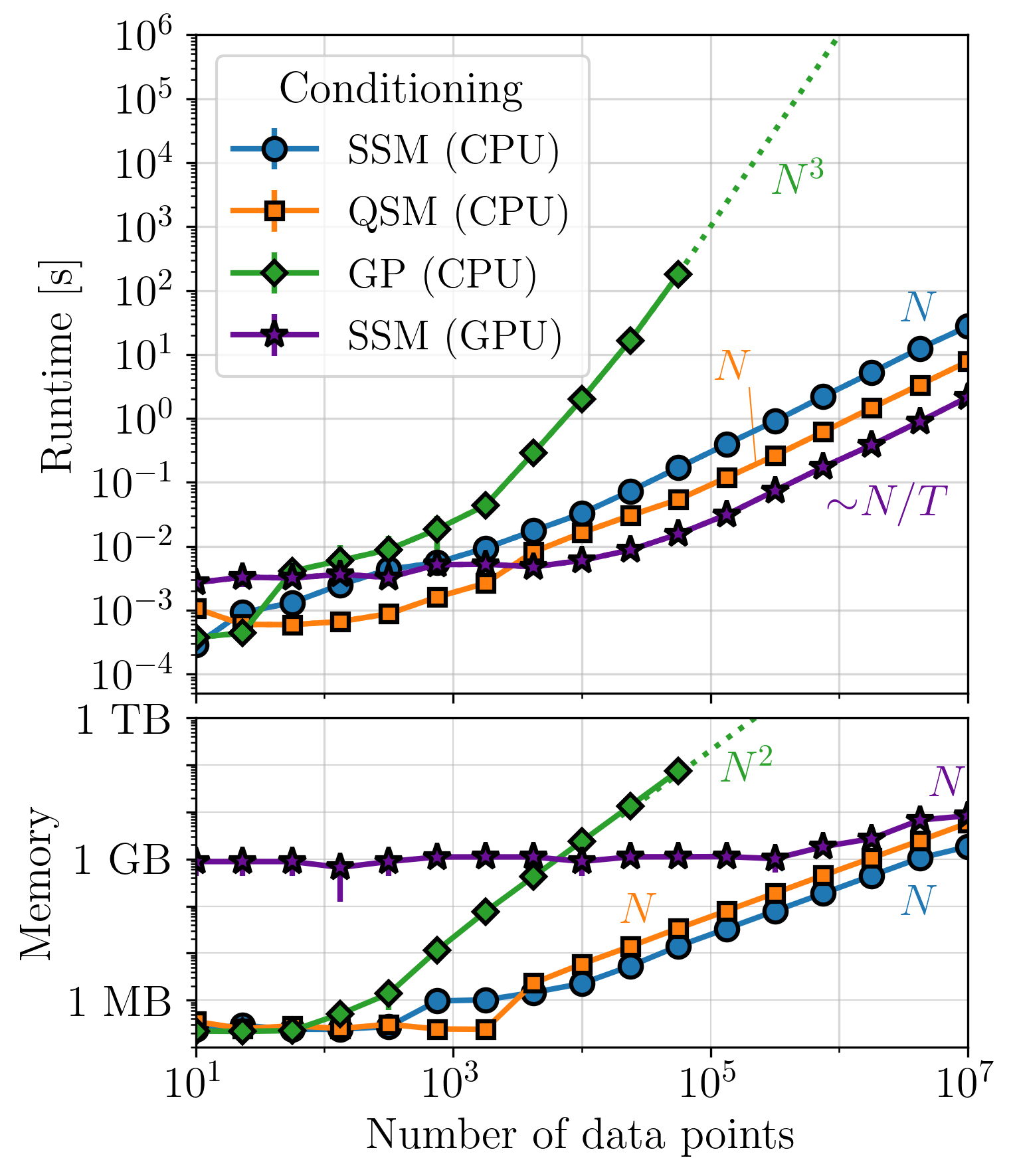
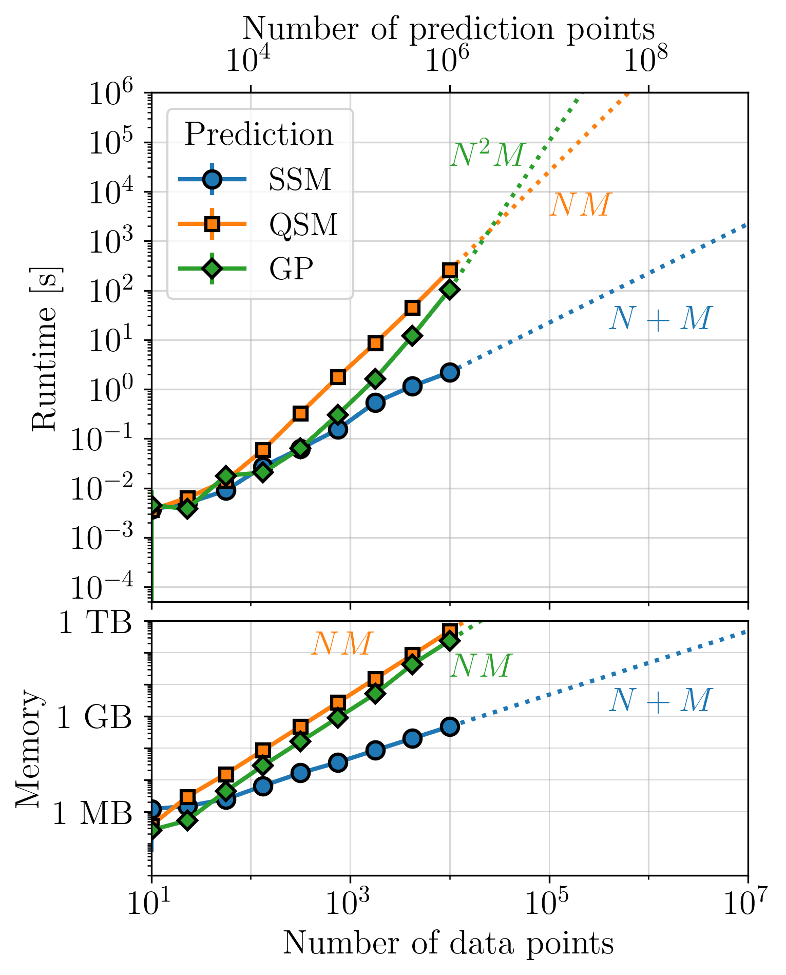
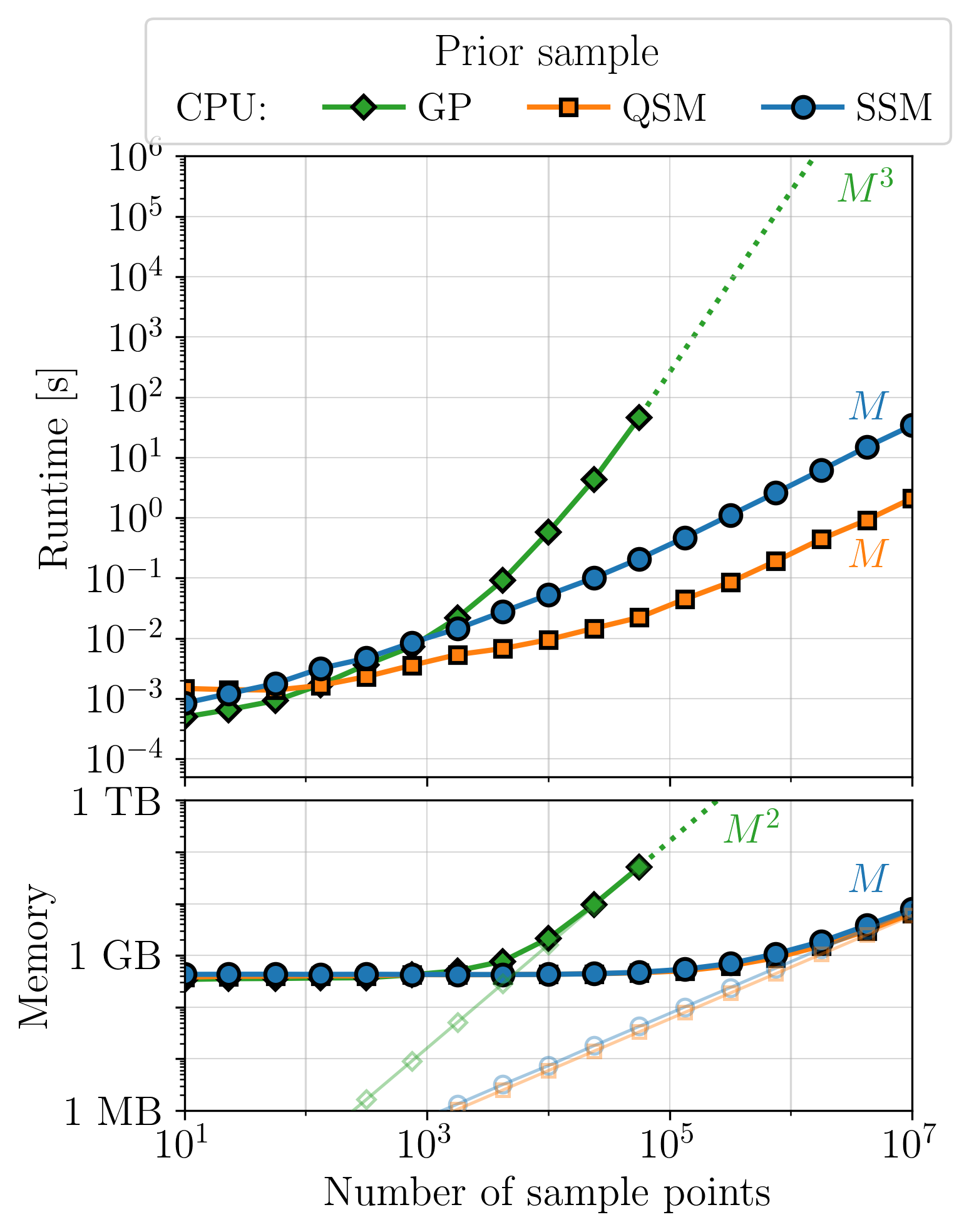
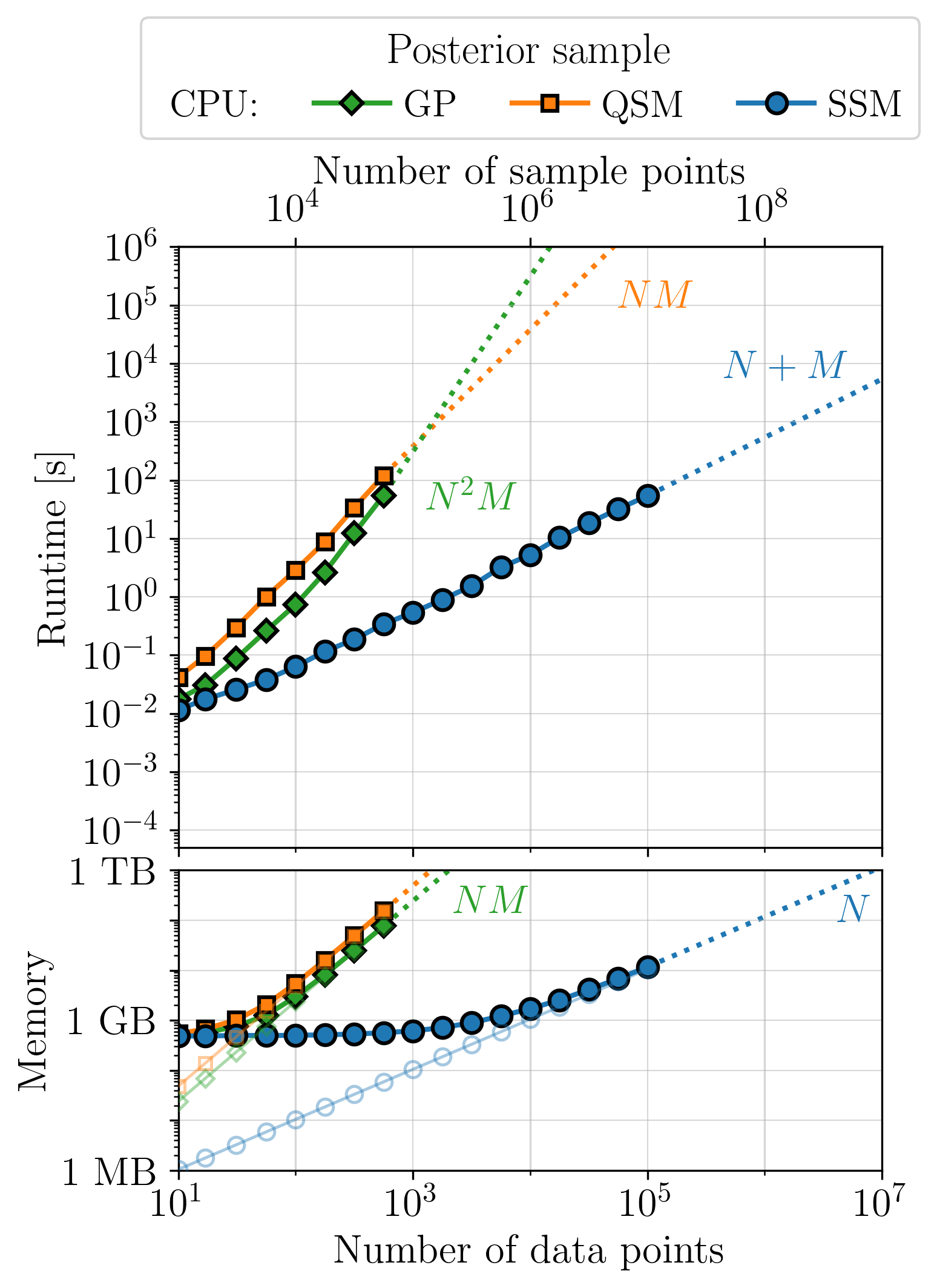
This page summarizes the key plots from Section 4 in Rubenzahl et al. 2026, which benchmark the performance of smolgp on CPU (blue curves) and GPU (purple curves). We compare to the performance of the full (dense) GP solution, as implemented in tinygp (green curves), as well as the tinygp quasiseprable implementation on CPU (orange) and GPU (red).

Each set of plots benchmark the runtime and memory usage for computing the

1. likelihood (value only and value + gradient)

2. conditioned mean and variance at the data points

3. predicted mean and variance at some test points,

4. drawing samples from the prior, and

5. drawing samples from the posterior.

Note that both predicting (#3) and sampling the posterior (#5) at test points scale with both the number of data points \(N\) and the number of test points \(M\). For simplicity, we fix \(M = 100N\).

Note

CPU benchmarks were run on an Intel® Xeon® w53435X with 512 GB RAM. GPU benchmarks were run on an NVIDIA RTX 6000 Ada with 48 GB of GPU memory, running CUDA v12.8. The functions used for timing and memory profiling are located in tests/benchmark.

For memory profiling, solid curves show the total peak memory the process actually used (i.e., including overhead like interpreter, JIT, etc.). The faded curves with open markers show just the memory used in the computation, taken from the XLA buffer.

Instantaneous measurements

For instantaneous measurements, and certain kernels[1], optimized quasiseparable matrix (QSM) algebra can be leveraged with tinygp to achieve similar-to-better performance as the state space method. However, kernels which do not have quasiseparable representations but can be approximated by a state space model, such as the quasiperiodic kernel, will see significantly faster performance in smolgp. In all cases, predictions with large datasets are substantially faster and less memory intensive with smolgp.

Integrated measurements

When the measurements individually span finite time intervals with variable length and/or overlap with other measurements, we cannot take advantage of any quasiseparable optimizations in tinygp and so are forced to use the \(\mathcal{O}(N^3)\) solution there. This is the scenario in which smolgp has the most impactful advantage over previous methods.

Note that sampling integrated exposures incurs an additional scaling penalty if the sample exposures overlap with one another, which goes cubically with the minimum number of “instrument” groups needed to describe the data with no self-overlaps.

---

[1]

Specifically the quasiseparable class of kernels implemented in tinygp.kernels.quasisep.